Modelling choices to manage crowds
How many different routes do you know to walk from your house to your nearest supermarket? Most likely, you can mention multiple slightly different routes. Yet, most people tend to prefer one or two routes to the remaining ones. The same is true for any choice you make as a pedestrian. We tend to have preferences. The better we understand why crowds prefer certain choices to others, the better we are able use this information to optimize crowd management procedures.
Underneath, we will first explain the basics of choice modelling, and accordingly showcase the two most used choice model types. To explain the theory, we will focus on pedestrian route choice.
Modelling choices
Any person makes hundreds of decisions each day. What to wear, what to eat, what activities to perform. While moving from A to B, we also make decisions, often subconsciously. Yet, understanding why we make choices helps us influence choice patterns of the crowd. Choice modelling is a way to do so.
In essence, choice modellers attempt to derive a mathematical description of the balance between factors that influence people’s choices. This mathematical description can accordingly be used to identify what pedestrians like (e.g. trees, entertainment), what they hate (e.g. rain, deviations), and what elements they are inert to. Understanding their balancing scheme helps us understand what we can do to influence their choices in a way that they align with our crowd management measures.
Capturing a choice in mathematics
Researchers capture people’s choice behaviour in order to capture people’s in mathematics. In order to do so, they ask large batches of people to:
Accordingly, they themselves
Based on these four elements, they use choice modelling procedures to distil the most likely explanation for the recorded choice of people in their sample. Train (2009) wrote a comprehensive introduction into the mathematical modelling of crowds.
The results of a choice model exercise is a mathematical description. For example, the made-up equation below.
Utility = -0.6 * distance + 0.1 nice pavement [0/1] + 0.02 * lux * female [0/1] + 0.1 * %trees + 0.05 * width pedestrian path
Here, one main assumption of the most dominant choice modelling frameworks is that people behave like a homo economicus. That is, people are consistently rational and narrowly self-interested and tend to maximize their utility. If the resulting utility (i.e. total experience or evaluation) of a certain route is higher, they are more likely to choose that route from their route set. If the resulting utility is lower, they are less likely to choose that route. Given that differences between people exist, the result is a choice probability, i.e. the likelihood to adopt a chosen route, and not a 100% certainty.
The sign of the equation illustrates whether we like or dislike certain characteristics of our choice alternatives. Using the example model before, this model shows that people:
Know these things, can help us design for pedestrians. For example, if we want all pedestrians to adopt the same route, we showcase one nice pedestrian route through the neighbourhood that limits walking distances to the main facilities, and has nice, smooth pedestrian paths that are well lit and feature many trees. If we want to ensure pedestrians distribute equally across the neighbourhood, we need to ensure that the utility of all routes are roughly equal.
A simple route choice model – the MNL
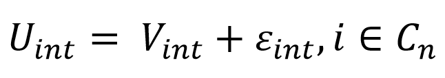
The most commonly used model to estimate pedestrian’ route choice is the Multinomial Logit (MNL) model, such as the one estimated by Casello & Usyukov (2014). The utility function for alternative i and observation n at time t specified in the following way (Ben-Akiva & Bierlaire, 1999):
(1)
Where V_in is the deterministic utility for alternative i (which is part of the choice set C_n) and observation n at time t and ε_int represents the random error term, which captures uncertainty and is independent and identically (i.i.d.) Gumbel distributed. The probability for an alternative to be chosen is calculated the following way:
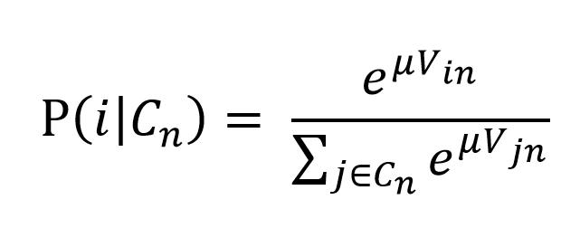
(2)
This model assumes that cyclists interpret each route as a distinct alternative (independence of irrelevant alternatives), while in reality the perception of routes that share common links might be correlated, implying that the MNL model will inadequately assign high probabilities to overlapping routes. The routes included in this study exercise some degree of overlap, therefore violating this assumption.
ASSIGNMENT 5.1 – route choice modelling
An engineer has estimated the following MNL model:
Utility = – 0.5 * distance[in km] + 0.2 * %route with greenery + 0.1 * %route lighted + 1.4 * safety score [1(worst)-5(best)]
Explain whether:
A. It is logical that the parameter for distance is negative.
B. It is logical that the parameter for safety is positive.
ASSIGNMENT 5.2 – True or false
For each of the following statements, determine whether they are true or false.
A. The alternative with the highest Utility is assigned 100% of the traffic demand
B. The variability of variables in a dataset has severe impact on the resulting model
C. The parameters of the MNL model can be compared directly. That is: U_1 = β_1 * X_1+ β_2 X_2, Therefore, β_2= 2 * β_1. Consequently, β_2 is 2 times more important than β_1.
D. The role of a constant in the utility function is to capture inexplicit bias for the alternative
E. MNL models can be used to model activity schedule choices, departure choice and route choices
ASSIGNMENT 5.3 – unravelling choice models
We have derived the following model.
Utility = – 0.5 * distance[in km] + 0.1 * %route lighted + 1.4 * safety score [1(worst)-5(best)] – 0.3 * average crowd density – 0.1 * number of turns
What would the nicest pedestrian route through a busy city centre look like according to pedestrians that make use of this utility function?
Incorporating overlapping routes
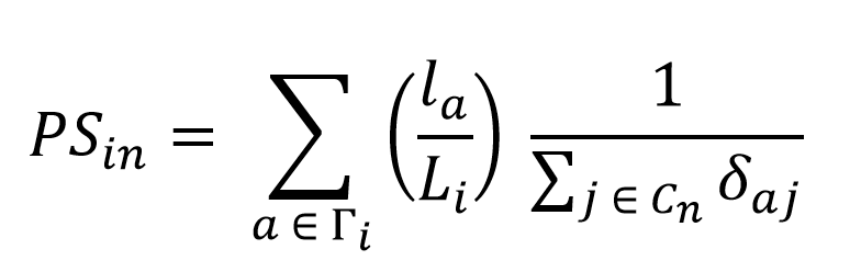
To account for overlapping routes, multiple solutions have been proposed in literature. The model structure applied in other cyclists’ route choice studies is the Path-Size Logit (PSL) model (e.g. Hood et al., 2011; Menghini et al., 2010; and Broach et al., 2012), which introduces a similarity measure in the utility function to account for the overlap. This approach maintains the MNL structure, making it easy to compute. For the calculation of the path size (PS) factor, different approaches have been put forward, however no straightforward answer can be provided to the question, which performs best. For example, the PS factors developed in a later stage can have illogical route probabilities (Freijinger & Bierlaire, 2007); whereas the earlier versions of the PS factor do not take large, differences in route length into account (Ben-Akiva & Bierlaire, 1999). In this course, we adopt the path size factor put forward by Ben-Akiva & Bierlaire (1999), because no large deviations in route lengths are present in the dataset:
(3)
where PS_in is the path size factor, Γ_i is the set of links in route i, l_a is the length (distance) of link a, L_i is the length of route i and δ_aj the link-route incidence variable which equals one if link a is on route j and zero otherwise. This means that the PS factor depends largely on the size and composition of the choice set (i.e. including many irrelevant routes affects this factor). The path size factor ranges between zero and one, where one indicates an independent route and zero indicates complete overlap with other routes in the choice set.
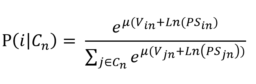
The probability for alternative to be chosen in the PSL model can be expressed the following way:
(4)
This means that the utility of overlapping alternatives (PS = 0) is slightly discounted by the path size factor. Thus, the probability of adopting these alternatives decreases (and as such the actual number of people choosing these alternatives) in comparison to the probability of the overlapping alternatives, when modelled by a ‘normal’ MNL model.
ASSIGNMENT 5.4 – Route overlap
We have the following two utility functions:
Utility1 = – 0.2 * distance[in km]
Utility2 = – 0.2 * distance[in km] + ln (Path Size factor)
Only Utility 2 accounts for the overlap. In addition, we have two routes, which both have a distance 10 km. The route comprises of 4 links, of which 3 are 100% overlapping.
A. Determine the utility per route and probability of choosing each route when overlap is NOT accounted for.
B. Determine the utility per route and probability of choosing each route when overlap is accounted for.
C. Determine how the probability would change if the overlap was still the same, but the length of the routes 20 km instead of 10.
D. Explain the difference in the utility of each route that you find.
E. Does the difference in utility also affect the route choice probability?
info@cityflows-projects.eu
Stevinweg 1, Delft, The Netherlands